Run multiple-pool models

Multiple-pool soil organic matter models are very useful to study dynamics that occur at different time-scales and that are controlled by different stabilization and destabilization mechanisms. A generalization of multiple-pool SOM models is given by the equation

$$ \frac{d{\bf C}(t)}{dt} = {\bf I}(t) + {\bf A}(t) \cdot {\bf C}(t), $$ which expreses how multiple soil carbon pools change over time as a function of external inputs and losses due to decomposition. In this model both inputs and decomposition rates can change over time.

In SoilR, multiple-pool models are implemented with the function GeneralModel. This function is a general constructor for any type of linear first-order model.

SoilR includes a set of functions that implement simple multiple-pool models. These functions are classified according to the figure below

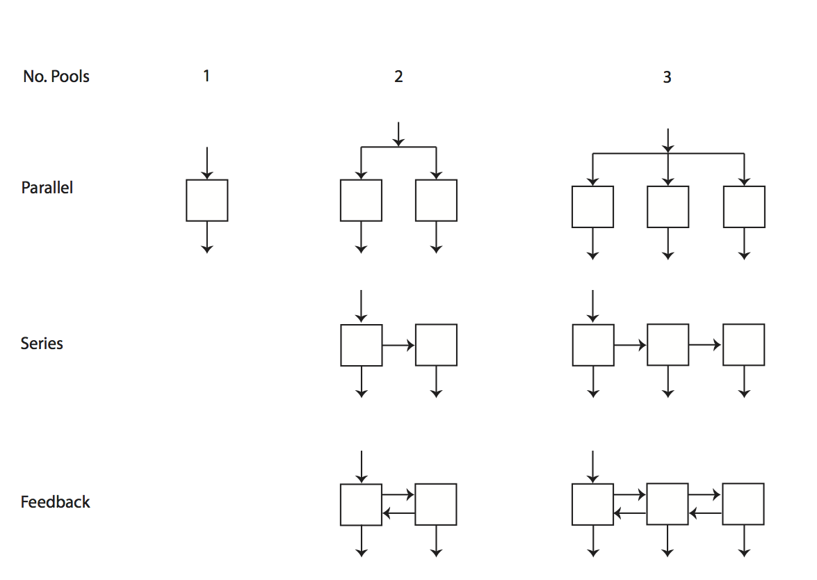
Functions TwopParallelModel, TwopSeriesModel, and TwopFeedbackModel implement the model structures represented above for two-pool models. Functions ThreepParallelModel, ThreepSeriesModel, and ThreepFeedbackModel implement the three-pool model structures above.

A three-pool model with feedbacks

As an example, we will implement a three-pool model with feedback assuming we have time varying litter inputs and temperature. The specific form of the model is

$$ \left( \begin{array}{c} \frac{dC_1}{dt} \\ \frac{dC_2}{dt} \\ \frac{dC_3}{dt} \end{array} \right) = \left( \begin{array}{c} I(t) \\ 0 \\ 0 \end{array} \right) + \xi(t) \cdot \left( \begin{array}{ccc} -k_1 & a_{1,2} & a_{1,3} \\ a_{2,1} & -k_2 & a_{2,3} \\ a_{3,1} & a_{3,2} & -k_3 \end{array} \right) \cdot \left( \begin{array}{c} C_1 \\ C_2 \\ C_3 \end{array} \right) $$

With initial conditions

$$ \left( \begin{array}{c} C_1(t= 0) = C0_1 \\ C_2(t=0) = C0_2 \\ C_3(t=0) = C0_3 \end{array} \right) $$

For the rate modifier we will implement a Q10 function of the form

$$ \xi(t) = Q_{10}^{(T(t)-10)/10}, $$

with Q10 = 1.4.

To implement the model, we need first to load SoilR in our R session

library(SoilR)

and create a vector of time steps to solve the model for this interval. We will create a sequence of 10 years in intervals of 1/12 (months)

t=seq(from=0,to=10,by=1/12)

For this example, we will create artificial data of litter inputs, assuming that every year an average of 10 Mg C/ha/yr enters the soil with an annual variability (standard deviation) of 2 Mg C/ha/yr.

Litter=data.frame(year=c(1:10),Litter=rnorm(n=10,mean=10,sd=2))
plot(Litter,type="o", ylab="Litter inputs (Mg C/ha/yr)")

Similarly, we will assume that daily measurements of temperature data are available for a period of 10 years. We will similute these data as

years=seq(from=1,to=10,by=1/365)
TempData=data.frame(years,Temp=15+sin(2*pi*years)+
                               rnorm(n=length(years),mean=0,sd=1))
plot(TempData,type="l", ylab="Soil temperature (Celcius)")

We can calculate the temperature effect on decomposition using the function fT.Q10 already implemented in SoilR. To use these results later, we will store the output in a data.frame.

TempEffect=fT.Q10(Temp=TempData[,2],Q10=1.4)
TempEffects=data.frame(years,TempEffect)
plot(TempEffects,type="l", ylab=expression(xi))

Now we need to specify parameter values and initial conditions

C0=c(C01=10,C02=40,C03=30) #Initial conditions for each pool

ks=c(k1=1/2, k2=1/5, k3=1/8) #Decomposition rates for each pool
a21=ks[1]*0.3 #Transfer coefficient from pool 1 to 2
a12=ks[2]*0.1 #Transfer coefficient from pool 2 to 1
a32=ks[2]*0.2 #Transfer coefficient from pool 2 to 3
a23=ks[3]*0.1 #Transfer coefficient from pool 3 to 2

We can now run the function ThreepFeedbackModel to initialize the model and check that parameter values, in particular the elements a, meet mass balance requirements. After initializing the model, we can calculate C stocks and release by pool with the functions getC and getReleaseFlux, respectively.

MyModel=ThreepFeedbackModel(years,ks,a21,a12,a32,a23,C0,
                            In=Litter,xi=TempEffects)
Ct=getC(MyModel)
Rt=getReleaseFlux(MyModel)

We can now plot the results for the carbon stocks

matplot(years,Ct, type="l", lty=1, col=1:3,ylim=c(0,max(Ct)), 
        ylab="Carbon stocks (Mg C/ha)", xlab="Time (years)")
legend("topright",c("Pool 1","Pool 2","Pool 3"),lty=1,col=1:3, bty="n")

and for the release fluxes

matplot(years,Rt,col=1:3, type="l", lty=1,  ylim=c(0,max(Rt)),
        ylab="Carbon release flux (Mg C/ha/yr)", xlab="Time(years)")
legend("topleft",c("Pool 1","Pool 2","Pool 3"),lty=1,col=1:3,bty="n")