Ages and transit times in linear models
Introduction
To compare different model structures or parameterization, it is useful to use simple diagnostic metrics about the rates of C cycling in soils. Two useful metrics are the transit time and the system age. These two metrics give an idea about the time required for molecules of carbon to travel through the soil system. In addition, we consider the concept of pool age, which is useful to determine cycling rates at the pool level. In this workflow we show how to compute these metrics for linear compartment models.
Definitions
We consider linear compartment systems of the form
$$ \frac{d{\bf C}}{dt} = {\bf u} + {\bf A} \cdot {\bf C} $$ where \({\bf C}\) is a vector of carbon stores, \({\bf u}\) is a vector of inputs to different pools. The matrix \({\bf A}\) is the decomposition operator, a \(n \times n\) compartment matrix where all the diagonal entries are nonpositive (the decomposition rates), off-diagonal elements are nonnegative (transfer rates among compartments), and all columns sums are nonpositive.
At steady-state, this system has solution
$$ {\bf C_{ss}} = -{\bf A}^{-1} \cdot {\bf u} $$
System and pool age
The system age is a random variable that describes the age of particles or molecules within a system since the time of entry. For linear compartment systems, Rasmussen et al. (2016) define the mean system age as
$$ E[A] = -{\bf 1}^T {\bf A}^{-1} {\bf \eta} $$ where \({\bf 1}\) is a column vector of 1, and
$$ \eta = \frac{ \mathbf{C_{ss}}}{\lVert \mathbf{C_{ss}} \rVert}. $$
The density function, not provided by Rasmussen et al. (2016), but derived by us (Metzler & Sierra 2018)
$$ f_A(y) = {\bf z}^T e^{y {\bf A}} {\bf \eta} $$
The pool age distribution is given by
$$ \mathbf{f_a}(y) = (\mathbf{X_{ss}})^{-1},e^{y,\mathbf{A}},\mathbf{u} $$
with mean pool age vector $$ E[\mathbf{a}] = -(\mathbf{X_{ss}})^{-1}, \mathbf{A}^{-1},\mathbf{C_{ss}} $$ where \(\mathbf{X_{ss}}\) is a diagonal matrix with the steady-state amounts.
Transit time
The transit time is a random variable that describes the ages of the particles at the time they leave the boundaries of a system; i.e., the ages of the particles in the output flux. It can also be interpreted as the time it takes for a particle to transit a system.
The mean transit time is defined by Rasmussen et al. (2016) as
$$ E[T] = -{\bf 1}^T {\bf A}^{-1} {\bf \beta} $$
where \({\bf \beta} = \frac{\bf u}{\lVert {\bf u} \rVert}\).
The transit time density function is given by
$$ f_T(t) = \mathbf{z}^T e^{t \mathbf{A}} \mathbf{\beta}. $$
Implementation in SoilR
Ages and transit times for linear compartment models are implemented in SoilR in versions older than 1.1-29 with the functions systemAge and transitTime.
For both functions, the arguments required are the matrix \({\bf A}\) and the vector of inputs \({\bf u}\). The matrix for any model
can always be derived from the system description (see Sierra et al. 2012).
Multiple-pool models
Consider as an example the following cases of pools models that have the same amount of inputs (100 units of mass per year) and the same stocks (1600 in units of mass)
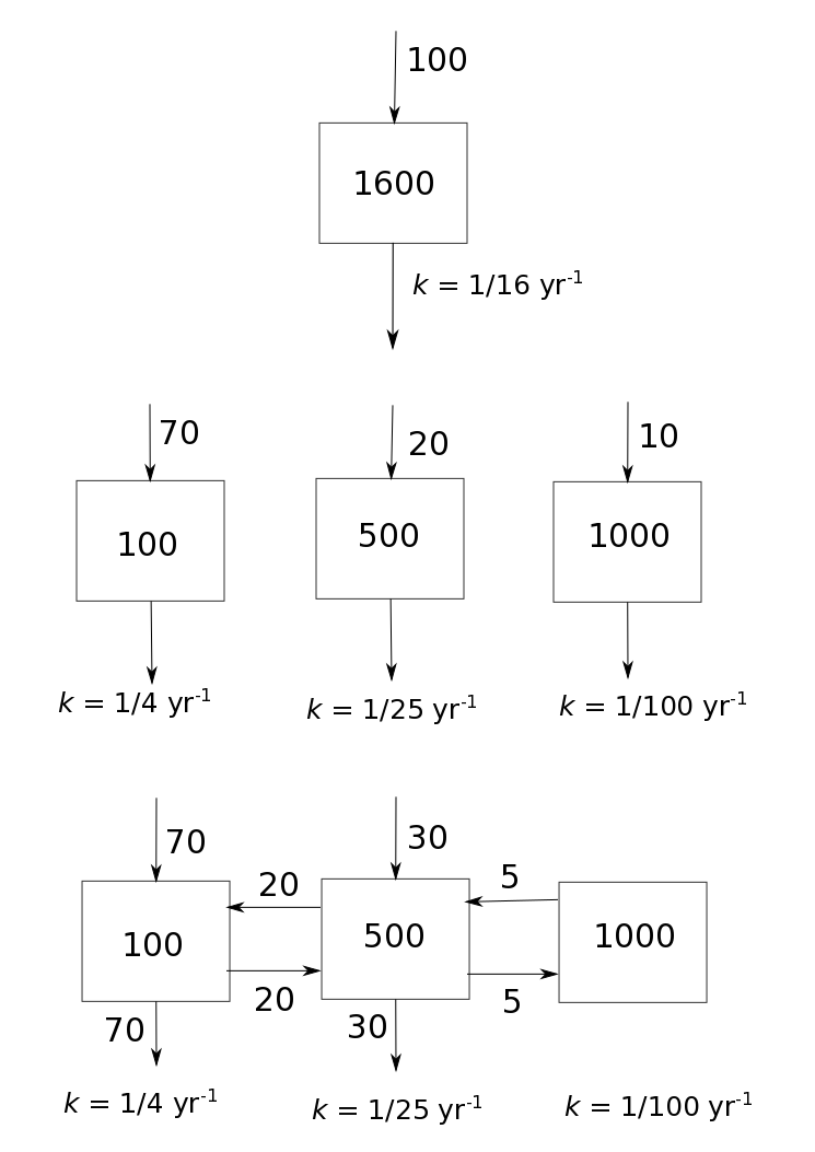
We can implement each model structure in matrix and vector form as
stock=1600
u1=100

k=c(1/4, 1/25, 1/100)
A2=diag(-k)
u2=matrix(c(70, 20, 10), ncol=1)

A3=diag(-k)
A3[2,1]=k[1]*(20/90)
A3[3,2]=k[2]*(5/(30+5+20))
A3[2,3]=k[3]
A3[1,2]=k[2]*(20/(30+5+20))
u3=matrix(c(70,30,0), ncol=1)
For the one-pool model at steady-state, the mean age and the mean transit time are the same and can be easily calculated as the stock over the input flux
SATT1=stock/u1
For the second model structure we calculate ages and transit times with SoilR functions as
SA2=systemAge(A=A2, u=u2)
TT2=transitTime(A=A2, u=u2)
and similarly for the third model structure
SA3=systemAge(A=A3, u=u3)
TT3=transitTime(A=A3, u=u3)
Now we can compare mean system ages and mean transit times for the two model structures
#Mean ages for the three models
SATT1
## [1] 16
SA2$meanSystemAge
##          [,1]
## [1,] 63.83146
SA3$meanSystemAge
##          [,1]
## [1,] 60.55396
#Mean transit times
SATT1
## [1] 16
TT2$meanTransitTime
## [1] 17.8
TT3$meanTransitTime
## [1] 22.35
Notice how different are the mean transit time and the mean ages for these different model structures even though they have the same amount of inputs, the same stock, and almost the same cycling rate.
We can also calculate the mean pool-age for each model structure
SA2$meanPoolAge
##      [,1]
## [1,]    4
## [2,]   25
## [3,]  100
SA3$meanPoolAge
##           [,1]
## [1,]  13.53659
## [2,]  42.91463
## [3,] 142.91463
Notice that the mean age of the pools differs from the turnover time of each individual pool in the case of the third model structure. This is due to the transfers of carbon among the different pools, which does not occur in the second model structure.
In addition to looking at the means, we can get additional insights by looking at the density distributions of ages and transit times.
par(mfrow=c(2,1))
plot(seq(0,100),SA2$systemAgeDensity, type="l", col=4, xlab="Age", ylab="Density function")
abline(v=SA2$meanSystemAge, lty=2, col=4)
lines(seq(0,100),SA3$systemAgeDensity, col=2)
abline(v=SA3$meanSystemAge, col=2, lty=2)

plot(seq(0,100), TT2$transitTimeDensity, type="l", col=4, xlab="Transit time", ylab="Density function")
abline(v=TT2$meanTransitTime, lty=2, col=4)
lines(seq(0,100), TT3$transitTimeDensity, col=2)
abline(v=TT3$meanTransitTime, lty=2, col=2)
legend("topright", c("Parallel structure", "Feedback structure"), lty=1, col=c(4,2), bty="n")

Although the differences in the distributions are relatively small, differences in the tails of the distributions contribute to large differences in the mean values.
Differences in the system age distributions can also be explained by the pool-age distributions. For the parallel model structure the pool age distribution is characterized by simple exponential functions:
par(mfrow=c(3,1))
for(i in 1:3){
  plot(seq(0,100),SA2$poolAgeDensity[,i],type="l",  ylab="Probability density", xlab="Age", bty="n")
}

For the feedback model structure the pool-age distribution take more complex forms that results from a superposition of exponentials.
par(mfrow=c(3,1))
for(i in 1:3){
  plot(seq(0,100),SA3$poolAgeDensity[,i],type="l",  ylab="Probability density", xlab="Age", bty="n")
}

Notice that the third pool in the feedback structure has much longer tails because a lower cycling rate and continuous recycling.
The Harvard Forest soil carbon model
A soil carbon model for the Harvard Forest was previously developed by Gaudinski et al. (2000), and tested in Sierra et al. (2012).
The matrix structure of this model is given by
ks = c(kr = 1/1.5, koi = 1/1.5, koeal = 1/4, koeah = 1/80,
       kA1 = 1/3, kA2 = 1/75, kM = 1/110)
A = -abs(diag(ks))
A[3, 2] = ks[2] * (98/(3 + 98 + 51))
A[4, 3] = ks[3] * (4/(94 + 4))
A[6, 5] = ks[5] * (24/(6 + 24))
A[7, 6] = ks[6] * (3/(22 + 3))
A[7, 2] = ks[2] * (3/(3 + 98 + 51))
A[4, 1] = ks[1] * (35/(35 + 190 + 30))
A[5, 1] = ks[1] * (30/(35 + 190 + 30))

LI = 150 #Litter inputs
RI = 255 #Root inputs
In=matrix(nrow = 7, ncol = 1, c(RI, LI, 0, 0, 0, 0, 0))
The mean and density distributions for ages and transit times can be obtained as
ages=seq(0,200) # Time vector for density functions
SA=systemAge(A=A, u=In, a=ages)
TT=transitTime(A=A, u=In, a=ages)
A plot of the density functions for age and transit time:
plot(ages, SA$systemAgeDensity, type="l", ylim=c(0,0.1), col=4,
     ylab="Density function", xlab="Age or transit time (years)")
abline(v=SA$meanSystemAge, lty=2, col=4)
lines(ages, TT$transitTimeDensity, col=2)
abline(v=TT$meanTransitTime,lty=2,col=2)
legend("topright",c(paste("Mean System Age = ", round(SA$meanSystemAge,2)),
                    paste("Mean Transit Time = ", round(TT$meanTransitTime,2))),
       lty=2, col=c(4,2), bty="n")

We can also see the density function for each pool
pools=c("Roots", "Oi", "Oe/a L", "Oe/a H", "A, LF (>80 um)", "A, LF (< 80 um)", "Min. Ass.")
par(mfrow=c(3,2))
for(i in 2:7){
  plot(ages,SA$poolAgeDensity[,i],type="l", main=pools[i], ylab="Probability density", xlab="Age", bty="n")
}

par(mfrow=c(1,1))
These density distributions clearly show how different the ages among and within pools might be. In particular, the slow cycling pools such as the mineral associated carbon present distributions with very long tails and a mix of new and very old carbon.